Lung Cancer Classification
Final Report
Project maintained by Bryan-Shook Hosted on GitHub Pages — Theme by mattgraham
7641 Final Report
1. Introduction / Background
Lung Cancer causes over 150,000 deaths each year, and it often goes untreated until severe symptoms begin which can often be too late. Currently, CT scans are used to discover Lung Cancer early, reducing mortality by up to 40% [1]. Recently, great strides have been made in the effectiveness of image classification using Neural Networks and specifically Deep Learning [3,7]. These advancements have made it feasible for Machine Learning to assist Medical Professionals in both detecting and classifying Lung Cancer from CT scans with similar or better accuracy and efficiency than before[6]. There have been a wide variety of attempts made to develop systems to do exactly that: detect and classify Lung Cancer from CT scans or other medical imaging[1,5]. It has been shown that Machine Learning systems have the ability to out perform radiologists by reducing variability and false-negatives[1].
In this project, we are using the LIDC-IDRI (Lung Image Database Consortium and Image Database Resource Initiative) dataset publicly hosted on The Cancer Imaging Archive. The LIDC-IDRI collection contains thoracic CT scans from over 1000 patients along with lung nodule annotations from expert radiologists. This data is stored in DICOM format comprising of 133 GB of data, suitable for use within scratch. Data set link: https://www.cancerimagingarchive.net/collection/lidc-idri/
2. Problem Definition
Despite gains from CT screening, early lung cancer still goes undetected because of subtleties and interobserver variability which still remains a challenge for cytopathologists [2]. The heavy volume and variability of manual review create opportunities for false negatives with serious cost. Our problem is to build a screening-support model that classifies CT images into cancerous and non-cancerous categories and flags potentially malignant nodules. Using the LIDC-IDRI CT dataset, we will test whether a CNN-based pipeline plus classical models can improve dianogistc performance without replacing radiologists.
Lung cancer is the leading cause of cancer death, and in screening settings, the harm of a false negative is high [4]. A high-recall, decision-support tool can surface attention to radiologists without disturbing their workflow. LIDC-IDRI offers a large, public, clinically relevant dataset to evaluate this tool. We aim to improve diagnostic consistency and safety while quantifying trade-offs for clinical usability.
3. Methods
Data Preprocessing
The dataset is a set of thoracic CT scans along with malignancy annotations rated 1-5 for each identified lung nodule. The dataset has several hundred thousand image slices. The preprocessing pipeline converts each image slice into a standardized 2D array. Pixel values are min-max normalized to [0, 1], converted grayscale if not already, and resized to 192px by 192px. We do this to remove any potential scanner intensity bias, and standardize data across scans.
We then apply a series of transformations: rotations, Gaussian blur, and normalization to 0.5 mean and 0.5 std. We also apply random flips to improve robustness and generalization. All samples are assigned binary labels, malignant is the annotation is greater than or equal to 3, and benign otherwise. We use an 80/20 stratified split by malignancy label to maintain class balance.
Model Architecture and Training
CNN
We first implemented a small convolutional neural network (TinyCNN as a PyTorch model class) to learn spatial and texture features from the CT slices. We decided on TinyCNN rather than a larger model such as ResNet in order to avoid overfitting from the limited slice of the dataset we used, it also allows for us to look specifically for nodule features. We start with 128x128 grayscale images, then we send it through 3 Convolutions. The first has 16 filters with a 3x3 kernel size, that is followed by a ReLU activation function and 2x2 Max Pooling. The second convolution is the same except it uses 32 filters, and then the Third uses 64 filters and negates the Max Pooling. The final feature map is put through AdaptiveAvgPool2s(1), which condenses the spatial information into a 64-dimensional feature vector. It outputs the dense feature vector for the later classifiers.
Optional Unsupervised Feature Augmentation
We hypothesize that the dataset might exhibit distinct groupings of nodules that could improve our classification performance if explicitly identified. To test this hypothesis, we applied K-Means clustering to the (64,) feature vectors extracted by the TinyCNN class. We only fit the K-Means algorithm on the training set features, and the validation samples were assigned clusters based on the learned centroids.
The cluster assignments were converted into one-hot encoded vectors and concatenated with the original TinyCNN features, resulting in output vectors of dimension 64 + N_CLUSTERS. These augmented output vectors were then used as the input for both the Random Forest and the Neural Network classifiers.
Random Forest
After getting the extracted features, we trained a Random Forest classifier from sklearn. Ensemble tree methods are good for feature spaces like CNN embeddings. Random forest has built-in regularization which can help with overfitting. In this project, we will use Random Forest to directly compare results with an end-to-end neural approach. It starts with the 64 features extracted by the Tiny CNN. It is optimized using a Log-Loss function, encouraging the output to be probability estimates. We use balanced class weights because our dataset is skewed in the number of malignant vs benign cases. We also try to penalize false negatives to a greater extent, as that is the goal of this tool. There are 500 estimators used to stabalize predictions and reduce variance. Note that, if using K-Means clustering, the input vectors are of the dimension 64 + N_CLUSTERS. If not using K-Means, the input dimension is 64.
Neural Network
We implemented a three-layer connected network (PowerfulFeatureNN as a PyTorch model class) on the same CNN embeddings to explore a more flexible classifier than Random Forest. The neural network
- Accepts the 64 +
N_CLUSTERSdimension input vectors if using the K-Means augmented feature set. If not using K-Means, the input dimension is 64. - Expands the feature space to 128, followed by batch normalization, ReLU activation, and 20% dropout for regularization
- Compresses back to 64 neurons followed by batch normalization, ReLU activation, and 20% dropout for overfitting.
- The output layer is a single neuron with sigmoid activation, producing a probability between [0,1] representing the likelihood of malignancy.
4. Results and Discussion
After performing Hyperparameter tuning to explore over 500 combinations of hyperparameters, we were able to determine hyperparameters that gave quite good results. Hyperparameter tuning was done primarily based off ROC-AUC of the CNN, Random Forest, and FC Neural Net models.
Feature Extraction (TinyCNN)
We first train the TinyCNN feature extractor in 40 epochs, resulting in the following learning curves (without K-Means, then with):

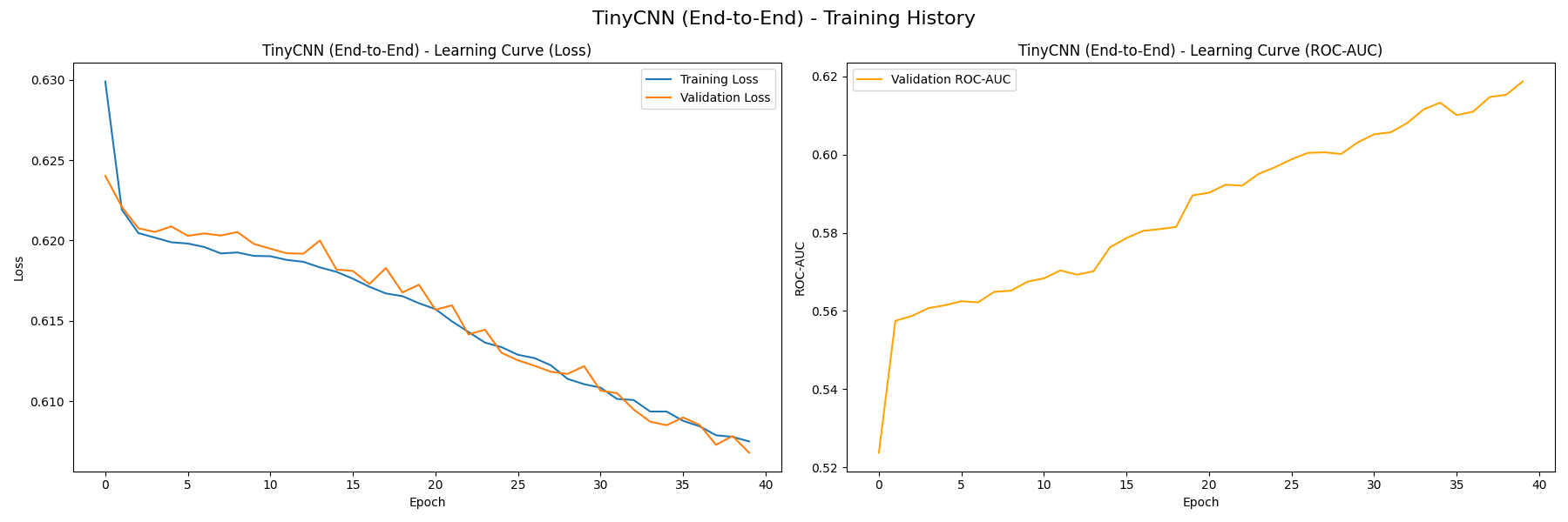 On the left plot, both the training loss and validation loss decrease steadily, which signifies that the model is not overfitting. We also measure the baseline performance of TinyCNN’s classifier using the curve on the right, which measures how the model’s ROC-AUC value grows with each epoch. The value grows from near 0.5 at initialization to approximately 0.62, signifying that the model is capturing useful patterns from the training data. You can see that there is very little difference between the version with/without K-Means, this likely indicates that our K-Means clusters don’t serve as valuable features to differentiate malignancy.
Random Forest Classifier
The classifier yields the following confusion matrix (without K-Means, then with):

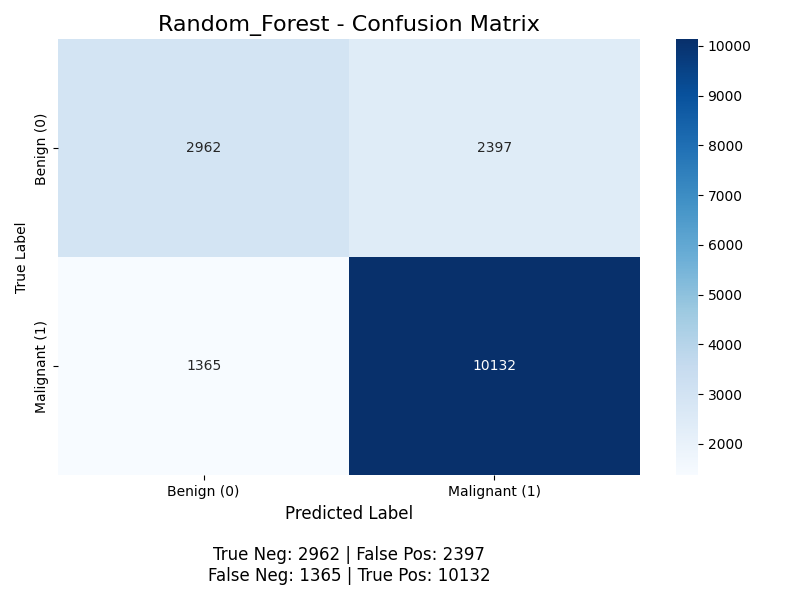 For positive classification (the “Malignant” class), the accuracy for without K-Means is (10126 + 2931) / (2931 + 10126 + 2428 + 1371) ≈ 77.5%, with K-Means it is (10132 + 2962) / (10132 + 2962 + 2397 + 1365) ≈ 77.5%, the precision is 10126 / (10126 + 2428) ≈ 80.7% without K-Means and 10132 / (10132 + 2397) ≈ 80.9% with K-Means, the recall is 10126 / (10126 + 1371) ≈ 88.1% without K-Means and 10132 / (10132 + 1365) ≈ 88.1% with K-Means (meaning the model successfully finds 88% of all malignant nodules), and the F1 score is 2 * (0.809 * 0.881) / (0.809 + 0.881) ≈ 0.843. The model achieves good performance, but its primary weakness is the 1365 false negatives with K-Means. With the Random Forests, we start to see some benefit from K-Means, but still very little.
The random forest classifier is able to perform better than the neural network classifier as it is more robust to noise and does not need a large dataset to generalize well.
Neural Network Classifier (PowerfulFeatureNN)
The classifier yields the following confusion matrix (without K-Means, then with):

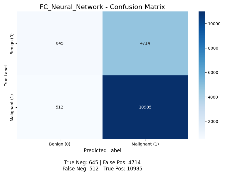 For positive classification (the “Malignant” class), the accuracy is (10955 + 666) / (10955 + 666 + 4693 + 542) ≈ 68.9%, the precision is 10955 / (10955 + 4693) ≈ 70.0%, but the recall is 10955 / (10955 + 542) ≈ 95.3% (meaning the model successfully finds 95% of all malignant nodules), and the F1 score is 2 * (0.700 * 0.953) / (0.700 + 0.953) ≈ 0.807. This model performs worse than the Random Forest Classifier, and we discuss potential next steps to improve this model below. With K-Means, its accuracy is (10985 + 645) / (10985 + 645 + 4714 + 512) ≈ 68.9%, the precision is 10985 / (10985 + 4714) ≈ 70.0%, but the recall is 10985 / (10985 + 512) ≈ 95.5% (meaning the model successfully finds 95% of all malignant nodules), and the F1 score is 2 * (0.700 * 0.955) / (0.700 + 0.955) ≈ 0.808. Same as before, we see a slight improvement from our K-Means, but the biggest thing we see here is that Recall is 95% while precision is 70%. This is interesting because if we are most worried about False Negatives, then this might work quite well. Though it does seem like its just learned that making the majority of reports Malignant works which might not be what we want. This is most likely because neural networks are more prone to over sensitive to class imbalance.
We also plot the ROC-AUC curves of all models as follows (without K-Means, then with):
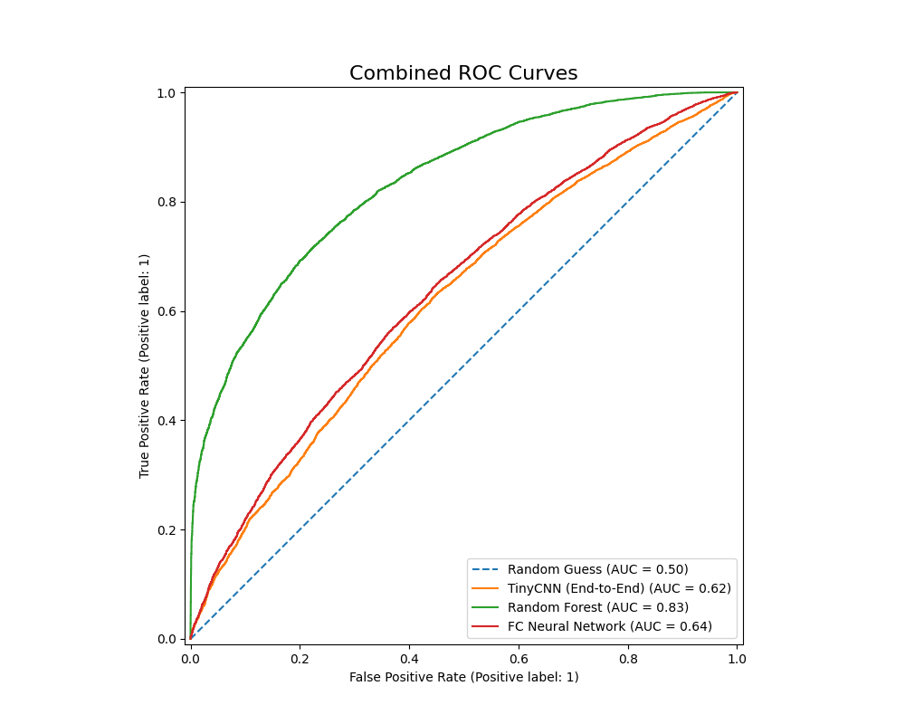
 The Random Forest classifer has an ROC-AUC value of 0.83, while the PowerfulFeatureNN classifier has a value of 0.640. This metric once again points to the Random Forest Classifier’s relative advantage given our current configurations: it has a higher accuracy, F1 score, precision, as well as better performance in differentiating between benign and malignant nodules. The Fully Conencted Neural Net however had a much higher recall, which might be ideal if we want to avoid False Negatives at all costs.
Next Steps
While there are many next steps we can take such as improving all hypermaraters and creating deeper models, the ultimate weakness lies in shallow feature extraction that that cannot exploit how rich and complex the image classification task truly is. To make meaningful progress beyond the current performance ceiling, we would need to rethink the entire pipeline and possibly introduce more techniques found in the literature. A first step would be to use deeper, pre-made models such as ResNet.
In summary, although small adjustments could refine our existing pipeline, our results show that real gains will come from replacing the pipeline with a stronger, clinically aligned architecture built on modern medical imaging techniques.
5. References
[1]D. Ardila et al., “End-to-end Lung Cancer Screening with three-dimensional Deep Learning on low-dose Chest Computed Tomography,” Nature Medicine, vol. 25, no. 6, pp. 954–961, May 2019, doi: https://doi.org/10.1038/s41591-019-0447-x.
[2]G. Acanfora, A. M. Carillo, F. D. Iacovo, et al., “Interobserver variability in cytopathology: How much do we agree?” Cytopathology, vol. 35, pp. 444–453, 2024, doi: 10.1111/cyt.13378.
[3]L. Schmarje, M. Santarossa, S.-M. Schroder, and R. Koch, “A Survey on Semi-, Self- and Unsupervised Learning for Image Classification,” IEEE Access, vol. 9, pp. 82146–82168, 2021, doi: https://doi.org/10.1109/access.2021.3084358.
[4]M. B. Schabath and M. L. Cote, “Cancer Progress and Priorities: Lung Cancer,” Cancer Epidemiol. Biomarkers Prev., vol. 28, no. 10, pp. 1563–1579, Oct. 2019, doi: 10.1158/1055-9965.EPI-19-0221.
[5]Q. Lv, S. Zhang, and Y. Wang, “Deep Learning Model of Image Classification Using Machine Learning,” Advances in Multimedia, vol. 2022, pp. 1–12, Jul. 2022, doi: https://doi.org/10.1155/2022/3351256.
[6]T. Kadir and F. Gleeson, “Lung cancer prediction using machine learning and advanced imaging techniques,” Translational Lung Cancer Research, vol. 7, no. 3, pp. 304–312, Jun. 2018, doi: https://doi.org/10.21037/tlcr.2018.05.15.
[7]W. Zhu, C. Liu, W. Fan, and X. Xie, “DeepLung: Deep 3D Dual Path Nets for Automated Pulmonary Nodule Detection and Classification,” 2018 IEEE Winter Conference on Applications of Computer Vision (WACV), Mar. 2018, doi: https://doi.org/10.1109/wacv.2018.00079.
Gantt chart files:
-
Excel: GanttChart.xlsx
Contributions
| Name | Final Contributions |
|---|---|
| Andrew Brown | Hyperparameter tuning pipeline |
| Bryan Shook | K-Means model implementation |
| Jason Yu | Report and Presentation Methods |
| Kai Hackney | Report Reports and Discussions, Hyperparameter tuning |
| Yash Agrawal | Classification structure modifications |